 Acad
AcadHow to Map Sentinel-2 NDVI in Python (No API Key)
How to map Sentinel-2 NDVI in Python usually means stitching together a STAC search, a cloud-optimised GeoTIFF reader, and a raster plotting stack — before you write a single line about your actual research. This post shows the honest full picture: what NDVI is, how to fetch and compute it from Sentinel-2, and how to do it with no API key, both the manual stackstac/rioxarray way and the one-line AcadGIS way.
What NDVI is and why researchers map it
The Normalized Difference Vegetation Index (NDVI) is the workhorse remote-sensing index for vegetation. Healthy plants reflect strongly in the near-infrared (NIR) and absorb red light for photosynthesis, so the contrast between those two bands tracks how much green, living vegetation is present. NDVI is defined as (NIR - Red) / (NIR + Red), which normalises the result to a fixed range from -1 to +1 regardless of overall brightness.
For Sentinel-2, the European Space Agency's 10 m optical mission, the red band is B04 and the near-infrared band is B08, so Sentinel-2 NDVI is simply (B08 - B04) / (B08 + B04). Researchers map it to monitor crop health, drought stress, deforestation, wetland extent and urban green space — anywhere a per-pixel measure of vegetation vigour turns satellite imagery into an analysable variable. Because both bands share the same 10 m native resolution, no resampling is needed and each Sentinel-2 NDVI pixel is a genuine 10 m ground measurement rather than an interpolated one.
NDVI value ranges and how to read them
Because NDVI is normalised, its values carry a consistent land-cover meaning across scenes and dates. The table below is the practical reference most analysts keep in their heads. Treat the boundaries as soft — atmospheric conditions, sensor angle and soil background all shift them by a few hundredths — but the ordering is reliable: water is negative, bare surfaces sit near zero, and dense canopy pushes toward one. This consistency is exactly why NDVI travels well between studies, and why a single legend can label maps from the Nile Delta to a boreal forest.
| NDVI range | Typical land cover | Interpretation |
|---|---|---|
| < 0 | Water, snow, cloud shadow | Non-vegetated; NIR reflectance lower than red |
| 0.0 - 0.2 | Bare soil, rock, sand, built-up | Little to no green vegetation |
| 0.2 - 0.5 | Sparse, senescent or stressed vegetation | Grassland, shrub, early crops or drought stress |
| 0.5 - 0.8 | Dense, healthy vegetation | Vigorous crops, temperate forest |
| 0.8 - 1.0 | Very dense canopy | Peak-season broadleaf forest, closed canopy |
Compute NDVI in Python with no API key
The key fact that makes this free is data access. Sentinel-2 L2A imagery is published as cloud-optimised GeoTIFFs on the AWS Open Data programme and indexed by the public Earth Search STAC catalogue (element84's earth-search.aws.element84.com/v1). That catalogue needs no API key and no login — you query it over plain HTTPS, unlike Google Earth Engine or the Copernicus Data Space, which both require authentication.
The honest manual route in pure ndvi Python code uses three libraries: pystac-client to search the catalogue for a scene over your area and date window, stackstac (or odc-stac) to lazily load the B04 and B08 bands into an xarray DataArray straight from the COGs, and rioxarray plus matplotlib to reproject, clip and plot. You compute NDVI as (nir - red) / (nir + red) once the bands are aligned. It works well and keeps you close to the data, but it is real plumbing: cloud masking with the SCL band, choosing a projection, handling nodata and picking a least-cloudy scene are all on you. Budget an afternoon the first time, then keep the notebook forever.
Map Sentinel-2 NDVI in one line with AcadGIS
AcadGIS wraps exactly that pipeline behind add_ndvi. It runs the Earth Search STAC query, pulls the red and NIR COGs, computes the index, mosaics the least-cloudy pixels over your window and draws the result — with no API key, because it uses the same open AWS catalogue. You give it an axis and an area, optionally a date range, and it returns a mapped NDVI layer on the standard RdYlGn ramp where green is high vegetation and red is bare or water.
The area is any region AcadGIS understands, so you can reuse the boundaries you already load for the rest of your figure. If you are building an orientation figure, this drops neatly into a study area map generator workflow alongside terrain and rivers, and the same call works whether your area is a single district or a whole country.
import acadgis as agis
gdf = agis.load_boundaries("Bangladesh", level="district")
ax = agis.plot(gdf, highlight="Dhaka", title="Sentinel-2 NDVI, Dhaka")
agis.add_ndvi(ax, "Dhaka", start="2024-03-01", end="2024-05-31", cmap="RdYlGn")
agis.save("dhaka_ndvi.png", dpi=300)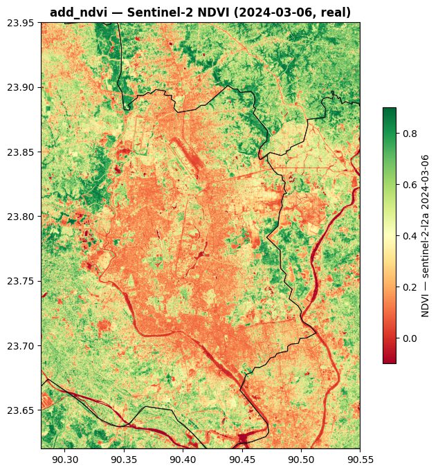
Choosing a date window and a clean scene
NDVI is a snapshot, so the start and end dates matter as much as the location. A wider window gives add_ndvi more Sentinel-2 passes to composite from, which helps it dodge clouds; a narrow window pins the index to a specific phenological moment, such as peak growing season or the height of a dry spell. For crop studies, choose a window inside the local growing season rather than the default full-year span, or you will average green-up and senescence into a muddy middle value.
Cloud is the perennial enemy of optical NDVI. Compositing over several weeks and taking the greenest or least-cloudy pixel per location is the standard defence, and it is why a season-long window usually looks cleaner than a single date. If your area is persistently cloudy — humid tropics, monsoon months — expect gaps, and consider a longer window or a drier month. Sentinel-2 revisits every five days at the equator with its two-satellite constellation, so even a three-week window typically stacks three or four passes to composite from.
Validating NDVI against ESA WorldCover land cover
An NDVI map is easier to trust when you can check it against an independent land-cover product. ESA WorldCover is a free global 10 m classification derived from Sentinel-1 and Sentinel-2, and it lines up pixel-for-pixel with your NDVI raster. Where WorldCover labels cropland or tree cover you expect high NDVI; where it labels built-up or bare ground you expect low NDVI. Disagreements are informative rather than embarrassing — they flag recently cleared land, seasonal fields caught out of season, or a cloudy scene that slipped through compositing.
AcadGIS exposes WorldCover through add_landcover, which reads the same open 10 m tiles, so you can render a land-cover panel beside your NDVI panel from one script. Because both layers accept the same area, this pairs naturally with a Python GIS mapping library figure that shows the index and its ground-truth classes side by side.
import acadgis as agis
gdf = agis.load_boundaries("Switzerland", level="country")
ax = agis.plot(gdf, title="ESA WorldCover 10 m, Switzerland")
agis.add_landcover(ax, "Switzerland", year=2021, legend=True)
agis.save("ch_landcover.png", dpi=300)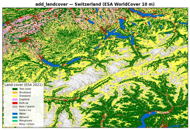
AcadGIS vs the manual stackstac route
Neither approach is universally better; they trade control for speed. The manual stackstac and rioxarray stack is the right tool when you need custom cloud masking, a specific projection, per-band scaling, or NDVI as an intermediate array feeding a model. AcadGIS is the right tool when you want a correct, publication-ready NDVI map now and would rather not maintain the STAC plumbing yourself.
It is worth naming the wider ecosystem honestly. geopandas handles vector boundaries but not raster indices; rasterio and rioxarray read the COGs; folium makes interactive web maps but is weak for static print figures; QGIS and ArcGIS can compute NDVI through a raster calculator but are not scriptable in a reproducible, one-file way. AcadGIS sits alongside these as a focused static-figure tool for journal-quality output. For a full physical-context figure you can layer NDVI with shaded relief from the terrain map generator.
| Step | Manual (pystac-client + stackstac + rioxarray) | AcadGIS add_ndvi |
|---|---|---|
| STAC search | Write pystac-client query against Earth Search | Handled internally |
| Load bands | stackstac / odc-stac loads B04 + B08 COGs | Handled internally |
| Compute NDVI | (nir - red) / (nir + red) by hand | Handled internally |
| Cloud handling | Manual SCL masking / compositing | Least-cloudy compositing over window |
| Plot + decorate | matplotlib styling, colorbar, extent | RdYlGn map, journal-ready |
| API key | None needed | None needed |
Exporting a publication-ready NDVI figure
Once the NDVI layer is on your axis, the last mile is resolution and annotation. Call agis.save("ndvi.png", dpi=300) to export at journal resolution, and because the whole figure is code you regenerate it instantly when a reviewer asks for a different season or a tighter crop. Add a north arrow, scale bar and title through the base plot call so the NDVI map reads as a finished figure rather than a raw raster dump.
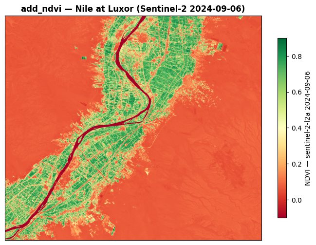
The result is a reproducible, single-file recipe: load your boundary, plot it, drop in add_ndvi, and save. No credentials, no desktop GIS session, and a full audit trail of exactly which dates and area produced the index — which is precisely what a methods section needs.
import acadgis as agis
gdf = agis.load_boundaries("Egypt", level="country")
ax = agis.plot(gdf, title="Sentinel-2 NDVI along the Nile at Luxor")
agis.add_ndvi(ax, "Luxor", start="2023-06-01", end="2023-09-30")
agis.save("nile_ndvi.png", dpi=300)Frequently asked questions
How do you compute NDVI in Python with no API key?
Compute NDVI in Python with no API key by reading Sentinel-2 L2A cloud-optimised GeoTIFFs from the public Earth Search STAC catalogue on AWS Open Data, which needs no login. Search with pystac-client, load bands B08 (NIR) and B04 (Red) with stackstac, and compute (B08 - B04) / (B08 + B04); or call AcadGIS add_ndvi to do all of it at once.
What is the NDVI formula for Sentinel-2?
For Sentinel-2 the NDVI formula is (B08 - B04) / (B08 + B04), where B08 is the near-infrared band and B04 is the red band. This is the standard (NIR - Red) / (NIR + Red) definition, and it yields values from -1 to +1.
What do NDVI values mean?
NDVI values below 0 usually indicate water, snow or cloud, 0 to 0.2 bare soil or built-up surfaces, 0.2 to 0.5 sparse or stressed vegetation, and above 0.5 dense healthy vegetation. The index is normalised, so these ranges hold consistently across scenes and dates.
Do you need Google Earth Engine to map Sentinel-2 NDVI?
No, you do not need Google Earth Engine to map Sentinel-2 NDVI. The imagery is free on the AWS Open Data programme and indexed by the Earth Search STAC catalogue, which is accessible over plain HTTPS with no account, so you can fetch and compute NDVI entirely in local Python.
How does AcadGIS add_ndvi avoid needing an API key?
AcadGIS add_ndvi avoids an API key by querying the public element84 Earth Search STAC catalogue and reading Sentinel-2 cloud-optimised GeoTIFFs directly from AWS Open Data, both of which are open and unauthenticated. It handles the search, band loading, NDVI computation and compositing internally.
How do you handle clouds when mapping NDVI?
Handle clouds by compositing over a multi-week date window and keeping the least-cloudy or greenest pixel per location rather than using a single date. In AcadGIS you widen the start and end range passed to add_ndvi; in a manual pipeline you mask with the Sentinel-2 SCL band before computing the index.