A Python GIS Mapping Library Built for Researchers Who Code

What a Python GIS mapping library is, and why researchers need one

A Python GIS mapping library is a package that reads spatial data (polygons, points, rasters) and renders it as a map you can drop into a paper, thesis or grant. geopandas and matplotlib already do this, but the everyday research workflow buries you in boilerplate: fetch and reproject boundaries, join a spreadsheet by region name, add a north arrow, place a scale bar, style a legend, then repeat it for every figure.

AcadGIS closes that gap. It is a thin, readable layer over the stack you already use, with defaults tuned for print. You are not learning a new GIS engine; you are calling a handful of functions that wrap geopandas geometries and matplotlib axes. Because it re-exports the whole ecosystem, agis.gpd.read_file() and agis.plt.subplots() are right there when you need to drop down a level.

Make a map in Python in a few function calls

The shortest useful program loads a country's administrative boundaries and plots them with academic styling. load_boundaries() returns an ordinary GeoDataFrame, so anything you know from geopandas still applies, and plot() adds a north arrow, scale bar and legend without extra arguments.

Because the import re-exports the ecosystem, you can filter, merge or compute with agis.pd and agis.gpd on the same object before it ever reaches plot(). When you need finer administrative detail, pass a different level or scope it with within= to a parent region.

import acadgis as agis

gdf = agis.load_boundaries("Bangladesh", level="district")
agis.plot(gdf, title="Districts of Bangladesh",
          theme="academic", north_arrow=True, scale_bar=True)
agis.save("districts.png", dpi=300)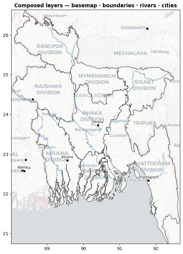

From tables to thematic maps

Most research figures are thematic: a value shaded across regions, or measurements plotted at sites. AcadGIS handles both. choropleth() takes a DataFrame or dict and fuzzy-matches your region names to the boundaries, so "Chittagong" still resolves to "Chattogram", then classifies with quantiles, natural breaks or equal intervals. If you want a click-free version of exactly this, the choropleth map generator wraps the same engine.

For point data (sampling stations, survey sites, gauges), points() draws onto any matplotlib axis, sizing or colouring markers by a column. Both functions return standard objects you can keep decorating with agis.plt.

import acadgis as agis

states = agis.load_boundaries("USA", level="state")
agis.choropleth(states, income_df, key="state",
                value="median_income", scheme="quantiles",
                palette="viridis", title="Median income by state")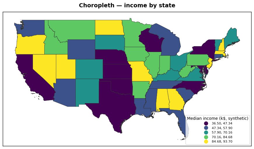

Terrain, satellite and study-area maps

Beyond boundaries, the library composes raster context. add_topography() and relief() render hillshaded elevation from Copernicus GLO-30, add_ndvi() pulls live Sentinel-2 imagery, and add_landcover() draws ESA WorldCover 10 m classes. Each targets a matplotlib axis, so you layer them in the order you want. See the terrain map generator for elevation-focused figures.

For the classic paper figure, a region set inside its national context, StudyArea and study_area() build cascade, inset and grid layouts in one call. The study area map generator covers that pattern end to end.

import acadgis as agis

fig = agis.StudyArea("Bangladesh", context_level="state") \
          .zoom_into("Dhaka", detail_level="district") \
          .figure(suptitle="Study area")
agis.save("study_area.png", dpi=300)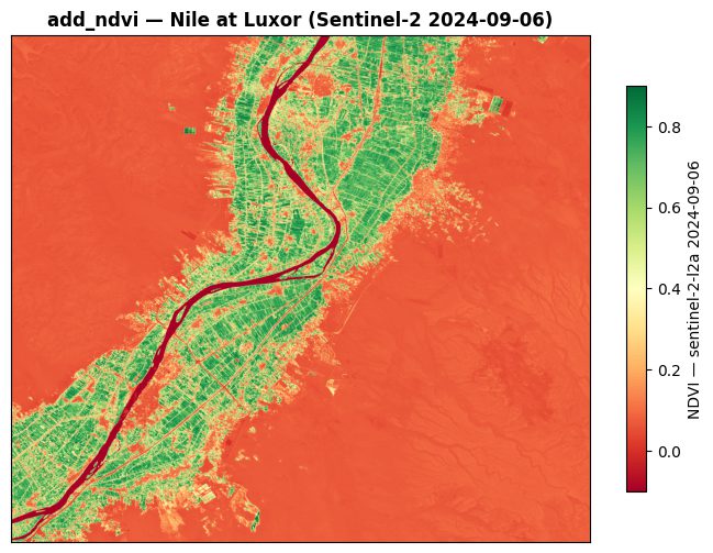

Concrete use cases across disciplines

The same handful of functions covers most figures a research paper needs. An epidemiologist maps case rates per district with choropleth() and fuzzy name matching, so a messy surveillance spreadsheet lines up with GADM boundaries without manual joins. A hydrologist overlays gauge readings with points() on a hillshaded basin from add_topography(), then traces the network with add_rivers(). An agronomist tracks crop vigour by dropping add_ndvi() over a study plot to pull live Sentinel-2 NDVI for a chosen date range.

Urban and ecology teams lean on the density tools: add_heatmap() for KDE or hexbin surfaces, dot_density() for population dot maps, and interpolate_field() with add_isopleth() for smooth contoured surfaces from scattered samples. Because every call hands back a real matplotlib axis, you can combine several in one composed figure for a methods section.

Data sources and practical tips

AcadGIS pulls from established open sources so your maps are citable: GADM for administrative boundaries, Natural Earth for coastlines and rivers, OpenStreetMap for roads, Copernicus GLO-30 for elevation, Sentinel-2 for NDVI, and ESA WorldCover for land cover. Bangladesh, Iraq, India and the USA are bundled and work fully offline; other countries download by name on first use.

A few tips: keep DPI at 300 for print with agis.save("fig.png", dpi=300); pass a colourblind-safe palette to plot() and choropleth(); and because every function returns a real geopandas or matplotlib object, you can always drop to agis.gpd or agis.plt for anything the wrappers don't cover.

Frequently asked questions